
/cloudfront-eu-central-1.images.arcpublishing.com/prisa/OJURMXSLDDF4EIPIOJG2SUZ3O4.jpg?w=1200&resize=1200,800)


Does a Joint Income Taxation System for Married
Abstract
This paper examines the impact of joint taxation of a married couple on the labour supply of women.I exploit reforms of the tax treatment of spouses that have occurred in 8 OECD countries, where elements of joint taxation have been replaced by separate taxation. Panel data and an event-study approach is used to estimate the causal effect on the female labour supply, which is positive but statistically insignificant. A micro-study on the tax reform in the United Kingdom is then carried out using Labour Force Survey (LFS) data and a difference-in-differences approach. Married women experienced a 4.1% increase in their participation rate and married women in the labour force experienced a 9.8% increase in total hours worked per week. There was an overall increase of 2.7 weekly hours of work for all married women.
1 Introduction
The income taxation system for a married couple can have distortionary effects on the labour supply of the secondary earner. The system implemented can either take the form of joint or separate taxation, where a separate system taxes each spouse’s income separately and a joint system taxes a married couple as a unit. Within a joint taxation system, pooled earnings are used to establish the marginal tax rate, which is equalised for both spouses and in effect reduced for the primary earner. As the marginal tax rate of the secondary earner is determined by the primary earner’s income, it is higher than it would be if they were taxed separately. Under neo classical assumptions, this disincentivises the labour supply of the secondary earner, which is in most cases the female in the couple. Therefore, economic theory predicts that joint taxation negatively affects the labour supply of married women.
This paper attempts to estimate the effects of joint taxation for married couples on the female labour supply using panel data and an event-study approach, which exploits several tax reforms involving a switch from joint to separate taxation using various treatment and control groups. OECD countries that have reformed their taxation system at differing points in time to remove elements of ‘jointness’ include Denmark, Sweden, the Netherlands, Austria, Finland, Italy, Belgium, Canada, Spain, and the United Kingdom. In the early 20th century, the traditional male breadwinner model defined most households in developed nations, in which the husband is the sole earner whilst the wife mainly focuses on domestic activities. When married women initially began to join the labour force, their earned income was perceived as an addition to the husband’s primary earnings and joint taxation
was used as the default system for most countries as a reflection of this principle. However, female participation in the labour market grew substantially in the mid 20th century and attitudes towards gender roles underwent significant transformation. Therefore, many developed countries have switched to a separate taxation system in an attempt to eliminate any gender bias and incentivise female labour force participation. This cross-country analysis finds a positive but not significant effect of separate taxation on the female labour supply.
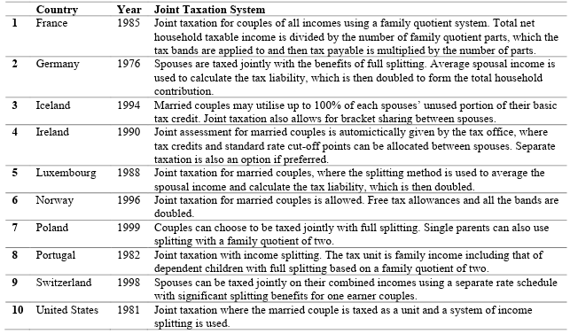
To provide a more in-depth analysis of the effect of joint taxation on the labour supply of married women, a micro-study on the United Kingdom is carried out using Labour Force Survey (LFS) data and a difference-in-differences approach. The UK switched to separate taxation in 1990. The previous system of joint taxation used meant that a married woman essentially had no independent status as a taxpayer, and her income was aggregated with her husband for tax purposes. After this was abolished, married women were assessed for income and capital gains tax as individuals. In theory therefore, this tax reform should have incentivised their labour supply. Their labour supply response is examined using measures at the extensive and intensive margin, which is positive and significant in all instances. At the extensive margin, married women experienced a 4.1% increase in their participation rate 5 years after the reform. At the intensive margin, there was a 9.8% increase in total hours worked over this time period. There was also an overall increase of 2.7 weekly hours of work for all married women. Joint taxation remains in place in France, Germany, Iceland, Ireland, Luxembourg, Norway, Poland, Portugal, Switzerland, and the US. It can either take the form of income aggregation or income splitting. Income aggregation is where the sum of family income is taxed as a whole. In France for example, income tax is assessed on the incomes of the whole household, which includes a married couple and dependent children living in the household, which enables larger families to pay less tax. Income splitting is where half a couple’s income is assigned to each spouse for tax purposes. For example, in Germany the system of ‘Ehegattensplitting’ enables a married couple to pay tax on their aggregate income. This creates tax savings for couples in which the primary earner has a considerably higher income than their partner and provides the most benefits for single-earner households. Therefore, there are large disincentives for the secondary earner to join the labour force. Joint taxation has been repeatedly criticised by the OECD and the EU commission due to the disincentive effects on the labour supply of married women. Furthermore, a recent statement from the European Parliament in 2019 urged member states to introduce individual taxation systems to achieve tax fairness and promote gender equality. Increasing female labour force participation is an explicit policy objective in many developed nations, as it is an important driver of economic growth and development. To achieve this, Governments often focus on policies that aim to minimise the impact of having children on the labour supply of women, such as childcare support and maternity leave entitlement. The tax treatment of married couples however is often omitted from the debate, despite being an influential factor. Therefore, there are clear policy implications from this research question if a move towards taxation on an individual basis can be shown to have significant positive effects on the female labour supply. The paper is organised in the following way: the next section considers the relevant literature. Next, the tax reforms to be exploited, the empirical strategy and the data used for this study are discussed. Then the empirical results are presented, and the conclusion lays out the policy implications.
2 Literature on Labour Supply and Taxation
A series of papers have examined labour supply responses of secondary earners, in particular married women. Blundell and Walker (1988) illustrate that a reform towards separate taxation for married couples, which reduces marginal tax rates for married women, has greater efficiency gains than a reform that reduces the marginal tax rate for the combined household. Kleven et al. (2009) determine the optimal income tax for couples, and more specifically how the tax rate on one individual should vary with the earnings of their spouse. Their findings support the notion of independent taxation, as optimal tax rates for secondary earners are below the marginal tax rates of primary earners. Kaygusuz (2010) investigates to what extent tax reforms in the US influenced the increase in the labour force participation of married women between 1980-1990 and finds that they account for 20-24% of the increase in the labour force participation rate of married women, and 27% of the increase in their working hours. Blau and Kahn (2007) find increasing labour force participation and decreasing labour supply elasticities of women over past decades, which suggests that estimated effects of joint taxation based on earlier reforms may be different to the effects nowadays.
Within the literature of labour supply responses to joint taxation, Bick and Fuchs-Schündeln (2017a) consider seventeen European countries and examine the effects of tax code progressivity and the tax treatment of married couples on married partners’ labour supply. This framework is built on in Bick and Fuchs-Schündeln (2017b) to quantify the disincentive effects of elements of joint taxation for married couples in these countries by analysing a counterfactual tax reform switching to entirely separate taxation. Their findings show that for all countries, married women would increase their labour supply as a result. The following papers provide evidence of the effects of joint taxation through changes in tax systems. Crossley and Jeon (2007) study a Canadian tax reform in 1988 which reduced the ‘jointness’ of the labour income taxation system and find that this significantly increased the labour supply of wives of high-earning husbands. LaLumia (2008) estimates the effect of the tax reform in the US in 1948 that switched from separate to joint taxation of married couples on their labour supply, using a natural experiment created by cross-state variation in property laws. This study finds a significant decline in the employment rate among women in highly educated couples. Kalíšková (2014) estimates the effect of the introduction of joint taxation in the Czech Republic in 2005 on married couples’ labour supply and finds a significant decrease in the employment rate of married women with children. Selin (2009) estimates the effect of the Swedish tax reform in 1971 switching from joint to separate taxation on female employment and finds that employment among married women would have been significantly lower if the system of joint taxation had continued. Isaac (2020) estimates the labour supply effects of joint taxation in the Untied States by exploiting tax variation created by federal same-sex marriage recognition, and finds that it significantly decreased labour force participation of lower earners. This paper contributes to this literature by broadly examining the effects of joint taxation on the female labour force participation at an aggregate level and more specifically estimating its effects on the labour supply of married women in the United Kingdom. To the best of my knowledge, there are no studies that provide evidence of labour supply responses to the switch to separate taxation in the UK in 1990.
3 Identifying Variation
This section identifies the relevant tax reforms to be exploited in the empirical analysis.
3.1 OECD Countries
Table 1: Tax Reforms in OECD Countries

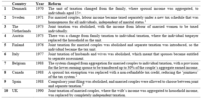
identified, however Denmark and Austria are later dropped from the sample due to data unavailability at the time of the reform.
In 1970, Greece was the only country in Europe to employ a system of separate taxation for married couples. Since then, many developed countries have moved away from a system of joint taxation to varying extents, in part because of the distortionary effects of on the labour supply of the secondary earner. This includes Austria, Belgium, Canada, Denmark, Finland, Italy, the Netherlands, Spain, Sweden, and the United Kingdom. These reforms can be used to obtain a causal estimate of the effect of switching to separate taxation on the female labour supply. Table 1 summarises the year of the reform in each country and what it entailed.
1An empirical analysis of this reform in Sweden can be found in Selin (2009). These findings show that employmentamong married women would have been 10% lower in 1975 if the 1969 system of joint taxation had continued.2This reform meant that the ‘first dollar’ marginal tax rate of the secondary earner no longer depended on the marginaltax rate of their spouse. Crossley and Jeon (2007) find a significant increase in labour force participation among marriedwomen to higher-income husbands after this tax reform in Canada. Their difference in-differences approach finds thatthe reform resulted in a 9 to 10% increase in the labour force participation of low-education women married to higherincome husbands. 3Fernández, et al. (2014) estimates the effect of the Spanish tax reform on the labour supply of married women. Theyfind the effect of the fiscal reform to be a 1.62% increase in labour participation.
3.2 The United Kingdom
Table 2: The 1990 Tax Reform in the United Kingdom

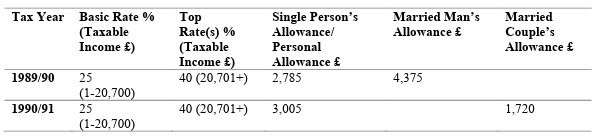
marginal rate. A single person received a Single Person’s Allowance (SPA). A married man benefitted from the Married Man’s
Allowance (MMA). A married women received a Wife’s Earned Income Allowance (WEIA) was equal to the SPA.
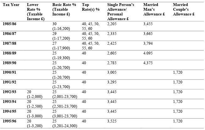
To provide a more detailed picture of the effect of joint taxation on the labour supply of married women, a micro-study on United Kingdom is carried out. In the UK, independent taxation of spouses came into effect on 6 April 1990. The previous joint taxation system treated the income of a married woman as if it were an extension of the income of the husband for tax purposes. Personal allowances were given as a deduction from the taxpayer’s income before the tax liability was calculated, and in effect gave relief at the taxpayer’s marginal rate of tax. A married man had a tax exemption in the form of a Married Man’s Allowance (MMA), which was just over one and a half times the Single Person’s Allowance (SPA), so couples stood to benefit financially from getting married as the man would receive a higher personal allowance. A married women who was working received a Wife’s Earned Income Allowance (WEIA), which was equal to the SPA, and her labour income (but not investment income) in excess of the allowance was taxed jointly with the income of her husband.
A system of independent taxation was proposed by Nigel Lawson, who stated in his 1988 Budget Speech that one of the main objectives was ‘to give married women the same opportunities for privacy and independence in tax matters as their husbands’. After the reform that came into effect in the 1990/91 tax year, each spouse was taxed separately on their labour and investment income.4 The other key element of the reform was the abolition of the Married Man’s Allowance. To avoid the household tax liability increasing for married couples (since the MMA was higher than the SPA), a new Married Couple’s Allowance (MCA) was introduced, which was equal to the difference between the SPA and the MMA. From 1990, everyone regardless of their sex and marital status was entitled to a Personal Allowance (PA) and married men additionally received the MCA. The change in personal allowances as a result of this reform are detailed in Table 2.
4Stephens Jr and Ward-Batts (2004) investigate whether there is a reallocation of asset ownership as a resulf of thisreform and they find evidence of a shift in investment income to the spouse with the lower marginal tax rate.
3.3 Changes in Marginal Tax Rates
Table 3: Household Labour Income Under the Pre-Reform Taxation System

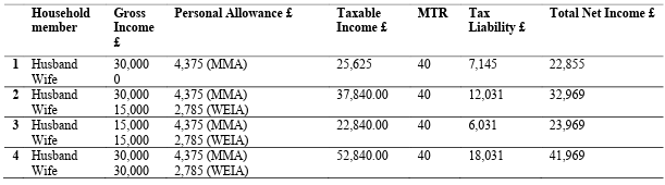
Notes: 4 hypothetical households in the tax year 1989/90. A married man benefitted from the Married Man’s Allowance (MMA). The
Wife’s Earned Income Allowance (WEIA) was equal to the Single Person’s Allowance (SPA).
Table 4: Household Labour Income Under the Post-Reform Taxation System

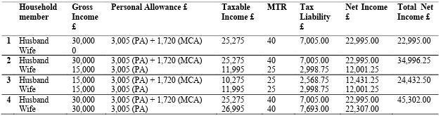
between the MMA and SPA. It was given to the husband but could be transferred to the wife if he was not making full use of it.
The abolition of joint taxation in the UK in 1990 created labour supply incentives for women married to high income men in the labour force. Table 3 and 4 illustrate how the tax liability would have been calculated for four different types of married couples in the tax year prior to and after the reform respectively. In 1989/90, the basic marginal tax rate of 25% was applied to taxable income, which is earned income above the personal allowance. The higher marginal tax rate was 40%, which applied to excess taxable income above £20,700. It was less likely for single people to pay tax at this higher marginal tax rate, and more likely for a dual income married couple, since the income of spouses was aggregated for tax purposes.
The first example considers a single earner married couple where the husband is part of the labour force and in the higher marginal tax bracket. As married women were entitled to the WEIA under joint taxation and the PA under separate taxation, the marginal tax rate was 0% on the very first pound of labour income earned both before and after the reform. Under joint taxation however, once their earned income exceeded this exempt amount, it was taxed at the MTR of their husband.
The second example considers a dual earning couple where the husband is in the 40% marginal tax bracket. In this instance, the entirety of the earned income of the wife in excess of her exemption was taxed at a 40% marginal rate. After the introduction of separate taxation, both spouses were taxed under the same income tax brackets, independent of each other’s earnings, so a married woman received the basic marginal tax rate of 25% on her earned income (above the exemption and below thehigher rate threshold), entirely independent of her husband’s income.
The third example refers to a two-earner married couple with equal incomes. Under joint taxation, if their aggregate taxable income exceeds the basic rate threshold (£20,700) then the wife would be in the higher marginal tax bracket of 40%, even if her husband was only in the 25% tax bracket. The introduction of separate taxation results in their incomes in excess of the personal allowance being separately taxed at the basic rate of 25%. Therefore, women benefited from separate taxation when their income was in the basic marginal tax bracket but considered to be in the higher bracket once it was added to their husband’s. The marginal tax rate of the wife would have been unchanged by the reform if the couple’s aggregate taxable income fell below this threshold. The fourth example shows that for a dual-earning couple with both partners on very high incomes, the marginal tax rate for both spouses is also unchanged by the reform. Therefore, for a group of married women whose marginal tax rate would have been reduced from 40% to 25% following the introduction of separate taxation, there would have been an incentive to increase their labour supply. Furthermore, after 1992 married women could receive a higher personal allowance, as they were eligible to be transferred all or half of the MCA from their husband if he was not making full use of it. The previous MMA penalised couples where the wife was a higher rate taxpayer, and her husband paid tax at the basic rate.
4 Empirical Strategy
4.1 Event-study of OECD Countries
The cross-country analysis is based on an event-study approach that exploits previous tax reforms that have occurred in various OECD countries. The ‘event’ is defined as the year in which the income taxation system for a married couple removes elements of ‘jointness’ in order to achieve a more individualised system. Details of these tax reforms can be found in Table 1. The labour supply response is examined at the extensive margin, with the outcome variable of interest the labour force participation rate. Various treatment and control groups are considered.
Table 5

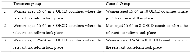
The estimate of the treatment effect of the tax reform is the difference between the change in labour force participation rate in the treatment group and the change in the control group. The comparison against a control group, which does not receive the treatment, allows the impact of the reform to be isolated from other factors, under the assumption that the labour supply response of the control group will provide a counterfactual outcome. Therefore, it is necessary that the control group is unaffected by the tax reform but is otherwise similar in its characteristics to the treatment group, which ensures that it is likely to respond similarly to the underlying trends. Since it is necessary for the control group to be similar in its characteristics to the treatment group, I have exclusively considered OECD countries, as the employment trends of women in these countries are similar. This method also requires that the pre-reform trends between the two groups are parallel for it to be plausible that the control group provides an accurate counterfactual result.
There are 10 OECD countries identified in Table 1 where a relevant reform took place, however Austria and Denmark are dropped from the sample since sufficient labour market data is unavailable in the time periods before and after. Therefore, there are 8 countries available to form the basis of the treatment group. A natural treatment and control group would be married and single women aged 15 64 within these countries. However, the dataset is unable to be broken down by marital status, so alternative control groups are identified. Table 5 details the various treatment and control groups that are instead used in the event-study. The first treatment group consists of women aged 15-64 within 8 countries that have moved towards separate taxation, and the control group consists of women aged 15-64 in 10 OECD countries in which joint taxation of married couples is still in place. Figure 1 in the Appendix shows that there are generally positive trends in the female labour supply across OECD countries, indicating that this will be a suitable control group. Figure 2 in the Appendix illustrates the female labour force participation rate in the treatment group for 5 years before and after the reform. Figure 3 in the Appendix shows the evolution of the female labour force participation rate in the 10 OECD countries in the control group, with a year randomly assigned in order to illustrate the reform.
These figures indicate that the parallel trends assumption is met, however this will also be empirically
tested. Table 6 in the Appendix details the joint taxation systems in place in the control group.
The following model is used to identify the impact of the tax reforms:
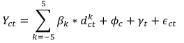

The dependent variable (!!») represents the percentage change in the female labour force participation rate relative to the year before the form, for country c at time t. The equation includes fixed country and fixed time effects ((! and )») to control for time-invariant group differences and for the common time trend in the labour supply. The impact of the reforms is captured by the estimators $#, which are the coefficients of the event-time indicator variables (&!» # ), where k indicates the number of years since the tax reform, and the omitted category is / = −1. For the event-study regression, 5 time periods are considered before and after the event, with the end points are binned up, and all of the countries in the control group are assigned / = −1.
An alternative control group is identified as men aged 15-64 in the 8 countries where the reform took place, under the assumption that men would not have adjusted their labour supply in response. Single men will naturally be unaffected by the reforms. Assuming that married men are mostly the primary earners, their marginal tax rates in some cases may have been raised after a switch to independent taxation. However, since estimates of male labour supply responses to tax changes are consistently found to be very small, the assumption can be made that these reforms would have had a negligible effect. Using this control group requires that employment trends of men and women evolve in the same way prior to the reform. Figure 4 in the Appendix illustrates the trends in female and male labour force participation within these 8 countries. As to be expected, the labour force participation rate is consistently higher for men than women. It also appears that the trends are parallel in the years leading up to the reform.
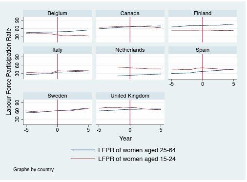
Another alternative method is to identify the treatment group as women aged 25-64 as the treatment group and women aged 15-24 as the control group. This is based on the assumption that younger women in this age bracket are much less likely to be married women in the older age bracket. This is plausible since at the start of the 1990s, the average age at first marriage across OECD countries was 25 for women.5 Figure 5 in the Appendix shows the labour force participation rates for younger women aged 15-24 and older women aged 25-64. The levels are much more similar for the two groups, and there is no clear pattern of either age group having higher rates overall. Again, it seems as though the trends are parallel in the pre-reform years, which is a necessary condition for this event-study.
5Source: OECD Family Database – Indicator SF3.1 – based on national statistical offices and Eurostat – http://oe.cd/fdb
For these variations, where the treatment and control groups are identified as different demographic groups within the same countries, equation 1 can be used to specify the model. Here, the dependent variable (!!») represents the first difference in labour force participation between the treatment and control group, for country c at time t. The advantage of using multiple control groups is that if the results are similar, it is more plausible that the estimated treatment effect accurately captures the effect of the tax reforms, and not just the effect of the other contemporaneous changes or trend differences between the control and treatment groups.
4.2 Micro-study of the United Kingdom
My empirical strategy to carry out a micro-study on the UK is based on a difference-in-differences method focusing on the reform in 1990, when joint taxation for married couples was replaced by separate taxation. The regression results are obtained using data from the Labour Force Survey between 1985 and 1995, in order to consider 5 time periods before and after the reform. Individuals excluded from the sample are those not of working age. The treatment group consists of married women aged 15-64 in the UK, as this group experienced changes in their marginal tax rates as a result of this reform. The largest change would have been for women married to men in the higher 40% marginal tax bracket, as their marginal tax rate on earnings above their personal allowance would have fallen from 40% to the basic rate of 25% after this reform. however, it is not possible to solely identify women whose marginal tax rate was affected by the reform as the treatment group since information regarding income and subsequent tax brackets is unavailable in the dataset. Single women aged 15-64 in the UK are identified as the control group as they are naturally unaffected by the reform. Therefore, this method therefore controls for any contemporaneous shocks to the labour force participation of women in the UK.
The first outcome of interest is the measure of labour supply at the extensive margin, using a dummy variable equal to one if the individual did paid work in the reference week. The measure of labour supply at the intensive margin response is also considered, using total log hours worked in the reference week in main and second jobs as another outcome of interest, conditioned on the individual having worked a positive number of hours. Total hours worked in the reference week is also considered as an outcome variable of interest, including women in the subsample that work zero hours, which provides an insight to labour supply responses at both the extensive and intensive margin. Control variables are used to control for other factors that are likely to determine an individual’s labour supply decision.
Two key identifying assumptions are made. Firstly, that there are no contemporaneous shocks (other than the tax reform itself) to the relative labour market outcomes of the treatment and the control groups in the same period of time as of the reform. This assumption is met since there were no other major changes to the UK taxation system going into the 1990/91 tax year. Table 7 in the Appendix details the income tax rates brackets and the personal allowances available in the entire time period considered. Secondly, the assumption is made that the change in the outcome of the control group is an accurate estimated counterfactual of the change in the outcome of the treatment group if the reform had not occurred. Therefore, it is necessary that the pre-reform trends of the treatment and control group are parallel to ascertain that the underlying trends do not differ between the two groups. Figure 6 in the Appendix illustrates the labour force participation rate of single and married women over the relevant time period, and it can be seen that before the reform, the trends between the two groups appear similar. This therefore presents some evidence for the validity of the parallel trends assumption at the extensive margin. This assumption also becomes more plausible once observable characteristics are controlled for. One way to empirically test this assumption is to compare the difference in outcomes between the two groups in the pre-reform years. Using the year before the reform as the base year, it can be tested whether the difference between the outcome of single and married women is significantly different to the base year in any of the other pre-reform years. If the common trends assumption holds, then there should be no statistically significant difference. The following model is used to identify the impact of the tax reform:
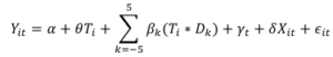

The dependent variable (!!») represents the outcome variable of interest for individual i at time t, either labour force participation or weekly hours of work. The equation includes a full set of year dummies and a treatment dummy, where 3′ takes a value 1 if the individual i is married and 0 otherwise. The impact of the reform is captured by the difference-in-difference estimators $#, which are the coefficients of the complete set of interactions of the treatment and time dummies, where k indicates the number of years since the tax reform, and the omitted category is / = −1. 6′» is a vector of additional covariates that control for observable differences in the characteristics of the treatment and control group that affect the individual labour supply choice. This includes dummy variables for age bracket (15-24, 25-34, 35-44, 45-54, 55-64), number of dependent children under 16 (none, one, two, three, four, and five or more), a dummy variable for race (=1 if non-white), and a full set of indicators for region of usual residence. Educational attainment is controlled for by a full set of indicator variables for different levels of highest qualification achieved (no qualification, GCSE equivalent, A-Level equivalent, other professional/vocational qualification, further education at or below degree level). A placebo test is also carried out by considering the male labour supply response to the tax reform at both the extensive and intensive margin. The difference-in-differences analysis is repeated with married men as the treatment group and single men as the control group, using the model specified in equation 2. Theoretically the labour supply of neither group should be altered as a result the abolition of joint taxation and therefore there no significant effects should be found. The marginal tax rate of single men will not be directly affected at all by the reform. The marginal tax rate of married men would have been largely unaffected due to the way in which the tax bill was calculated under joint taxation. Prior to the reform, a married woman’s labour income exceeding her personal allowance was added to her husband’s income for tax purposes. Therefore, taxing spouses separately would affect the marginal tax rate of the wife more than the husband, assuming the husband is the primary earner. Furthermore, estimates of male labour supply responses to tax changes are consistently found to be very small. Both Kalíšková (2014) and LaLumia (2008) find mostly insignificant effects of joint taxation on the labour supply of married men. Figure 7 in the Appendix illustrates the labour force participation rate of single and married men over the relevant time period. This shows that the trends for married men and single men evolve in the same way over time and do not appear to be altered by the reform.
5 Data
5.1 Event-study of OECD Countries
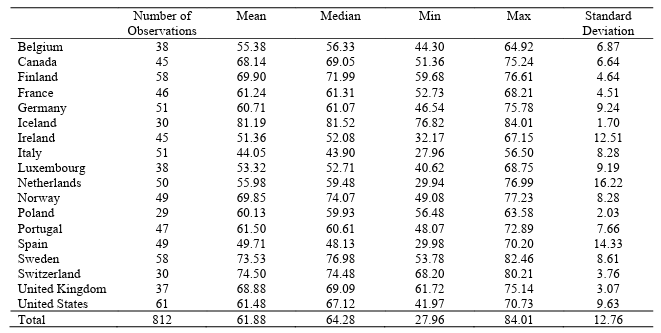
I use the OECD Employment and Labour Market Statistics database, which includes annual labour market statistics and indicators from 1960, to obtain an unbalanced panel of 20 OECD countries.6 This contains the annual labour force participation rates and can be separated by gender and age group, but not by marital status. Since the reforms of interest occurred at various points in time for different countries, data is obtained for the years 1960 2020. However, data is less widely available in the earlier decades. Therefore, although 10 countries are identified with relevant tax reforms, 2 countries (Denmark and Austria) are dropped from the sample due to data being unavailable around the time of the reform. Table 8(a) in the Appendix summarises the female labour force participation rates in all of the countries considered. Table 8(b) in the Appendix summarises the labour force participation rates in the other demographic groups used in the alternative treatment and control groups.
6OECD (2021), «Labour Market Statistics: Labour force statistics by sex and age: indicators», OECD Employment andLabour Market Statistics (database), https://doi.org/10.1787/data-00310-en (accessed on 01 December 2021).
5.2 Micro-study of the United Kingdom
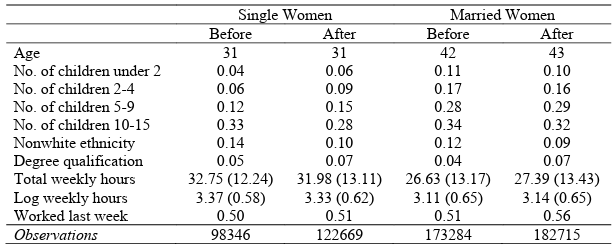
Table 9: Summary Statistics by Treatment Group and Period


The pre-reform period is defined as 1998-1989 and the post-reform period is defined as 1990-1995, since independent taxation was
introduced in 1990. Source: UK LFS data. For total and log weekly hours worked, only women working between 1-75 weekly hours
are included, with standard deviations in parenthesis.
To examine the labour supply of women in the UK, I use the UK Labour Force Survey, which began in 1973 and surveys roughly 100,000 households.7 I will use this survey to provide repeated cross sectional data for a sample of women and men aged 15-64 from 1985-1995. Since the reform occurs in 1990, I use data from the five years prior to the reform and the five subsequent years. This survey contains information about the composition and demographic characteristics of the household, their economic activity and the number of weekly hours worked. Table 9 reports averages of the main outcome and control variables by treatment group and treatment period calculated from the LFS data. It can be seen in this table that married women are on average older, more likely to have children, and work less hours. Their participation rates surpass those of single women after the reform, where 51% of married women have completed paid work in the reference week in the pre-reform period, which increases to roughly 56% in the post-reform period. Similar patterns can be seen for men in the sample in Table 9(b) in the Appendix. Married men have the highest labour force participation rates and average weekly hours than all other groups, with roughly 77% having worked that week.
6 Empirical Results
In this section, I present the main estimation results of the female labour supply response to separate taxation from the event-study of OECD countries and the micro-study of the United Kingdom.
7 Office of Population Censuses and Surveys, Social Survey Division. (2004). Labour Force Survey. UK Data Service.
6.1 Event-study of OECD Countries
Figure 8: Regression results

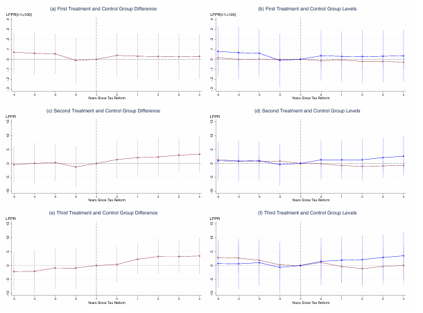
groups previously detailed in Table 5. These figures plot the regression coefficients from the event-study regression modelled in equation
1 and their respective confidence intervals. In Figure 8(a) and Figure 8(b), the labour force participation rate is normalised at 100 at the
year before the reform !−1. Figures 8(a), 8(c) and 8(e) detail the difference between the change in labour force participation rate of the
treatment and control group, and Figures 8(b), 8(d) and 8(f) show the respective levels of the two groups. The blue lines represent the
change in LFPR relative to !−1 for the treatment groups and the red lines represent the control groups.
Figure 8 shows that overall, there is no statistically significant difference between the change in the labour force participation rate of the treatment group and control group. However, the effect is always positive, which shows that the labour force participation rate of the treatment group always increased more than the control group after the reform. This effect is clearer for the second and third treatment and control group variations, when these groups are identified as different demographic groups within the same countries. Figure 8(c) shows the difference between the change in the LFPR for women and men relative to the year before the reform. This remains very close to zero before the reform and becomes increasingly positive afterwards, although still insignificant. Figure 8(e) shows a very similar trend for older and younger women. The treatment effect on married women is unable to be observed from the dataset, so the results could be masking heterogeneity between married and single women. Table 10 in the Appendix details the regression coefficients and their standard errors.
6.2 Micro-study of the United Kingdom
Figure 9: Regression Results Measuring Labour Supply at the Extensive Margin

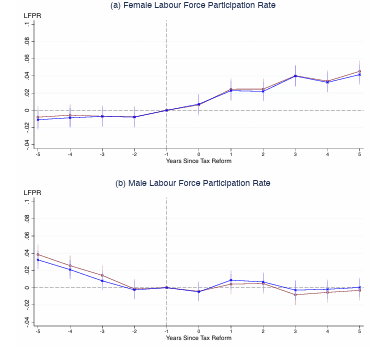
is considered, spanning from 5 years before the reform and 5 years after. The dots represent the difference-in-differences coefficients
(the interaction of the treatment dummy with post-reform years) from equation 2 and the lines represent their 95% confidence intervals.
The red line gives the results without control variables, and the blue line shows the results after controlling for observable characteristics.
Figure 9(a) shows the impact of the UK reform in 1990 on the labour force participation rate of married women. The regression coefficients indicate the change in the difference in labour force participation between married and single women relative to the year before the reform. The coefficients are all insignificantly different from zero for the years before the tax reform, which provides evidence for the parallel trends assumption, since it shows that the difference between married and single women does not change in the years leading up to the reform. The effect is positive but not significant for the year 1990, which is a partially treated year as it is the year in which the reform came into effect. The effects are positive and significant for all post-reform years, which shows separate taxation had a positive effect on the labour force participation rate of married women. Including control variables in the regression has noticeably little impact on the outcomes. Figure 9(b) gives the results when the same regression is carried out for men in the sample as a placebo test. The results are all insignificant after the reform, which is to be expected as the labour supply of men is unlikely to be affected. There are some significant results in the early pre-reform years, however they are of a smaller magnitude, and this effect is slightly reduced by controlling for observable characteristics.
Figure 10: Regression Results Measuring Labour Supply at the Intensive Margin

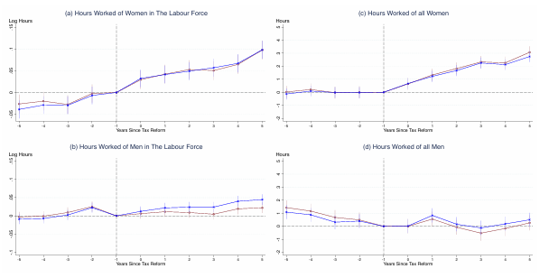
from 5 years before the reform and 5 years after. The dots represent the difference-in-differences coefficients (the interaction of the
treatment dummy with post-reform years) from equation 2 and the lines represent their 95% confidence intervals. The red line gives the
results without control variables, and the blue line shows the results after controlling for observable characteristics.
Figure 10 shows the labour supply response to the UK reform at the intensive margin. The regression coefficients indicate the change in outcomes between married and single women relative to the year before the reform. Figure 10(a) illustrates the results for women in the labour force using log weekly hours worked as the outcome variable of interest. The coefficients are generally insignificantly different from zero for the years before the tax reform, although in some cases they are negative and significant, but of a small magnitude. The effects are positive and significant for all post-reform years and including control variables in the regression has noticeably little impact on the outcomes. Figure (c) uses total weekly hours worked for all women in the sample (including those who work zero hours) as the dependent variable, in order to capture an extensive and intensive margin response. The coefficients are all very close to zero for the years before the tax reform, which provides evidence for validity of the parallel trends assumption, and positive and significant in the post-reform years. Figures 10(b) and 10(d) show the results of the same regressions carried out for men. In Figure 10(b), the effects are generally insignificant in the pre-reform years, and in the post-reform years there are some positive and significant results, which suggests married men already in the labour force slightly increased their hours compared to their single counterparts. The results are generally insignificant after the reform in Figure 10(d), and there are some significant results in the early pre-reform years of a small magnitude.
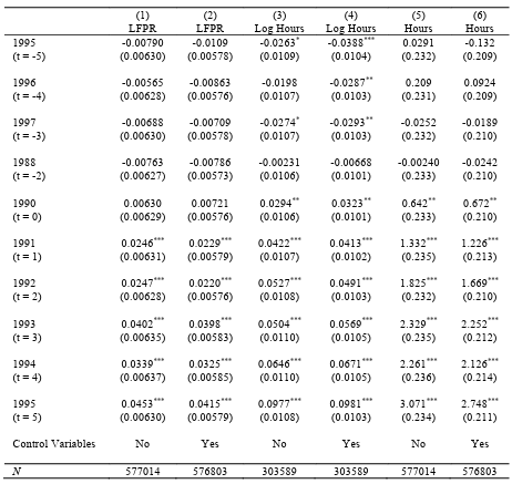
Table 11: Labour Supply Response to Separate Taxation of Married Couples

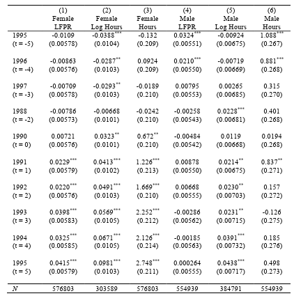
Notes: Robust standard errors in parentheses. * p < 0.05, ** p < 0.01, *** p < 0.001. This table presents the regression results illustrated
in Figures 9 and 10, where control variables are included. The base year is the year before the reform (1989).
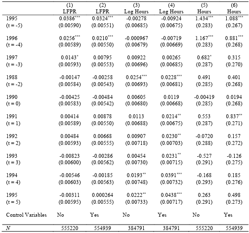
Table 11 reports the difference-in-differences coefficients from equation 2 and their robust standard errors. The coefficients of the interaction variables represent annual deviations from the difference in outcomes between married and unmarried females, relative to the year before the reform (1989). Labour supply is considered at the participation margin, measured by whether paid work was carried out in the reference week, and at the intensive margin, measured by log hours (for all working individuals in the sample). Total hours are also used as a measurement for all individuals in the sample, which records a labour supply response that captures both the extensive and intensive margin. Columns 1-3 show that the effect on the labour supply of married women of the reform is positive and significant by all measurements. The coefficient of 0.0415 in column 1 shows that 5 years after the reform, married women experienced a 4.1% increase in probability of working. For married women who worked a positive number of hours in the reference week, there was a 9.8% increase in total hours worked. There was also an overall increase of 2.7 weekly hours of work for all married women. Columns 4-6 display the results when the same regressions are carried out for men in the same sample. The results are generally insignificant, which shows that there was little effect on their labour supply. There are positive and significant results at the intensive margin, but of a smaller magnitude than for women.
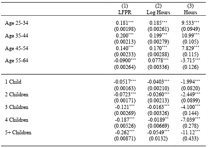
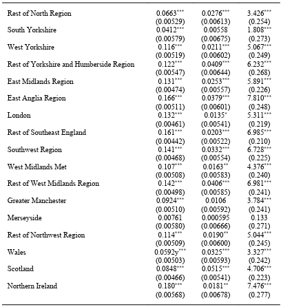
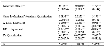
Table 12 in the Appendix details the full regression coefficients and their standard errors for the outcome variables of interest and the control variables used. The regression coefficients on the control variables all take the expected signs and are similar for men and women. The age band associated with the highest levels of labour supply is 35-44. Being of a non-white ethnicity has a significantly negative effect on labour supply. Having more children has an increasingly negative effect for both genders, but it is stronger for women. Residing in different regions also has significant effects on labour supply. Also, having a higher qualification is associated with higher levels of labour supply.
6.3 Extensions
Further considerations can be made about the type of work that was taken up. Figure 11 in the Appendix illustrates the results when work is categorised by part time and full time. This reveals that married women experienced a significant increase in likelihood of working fulltime, whilst the likelihood of completing part time work did not significantly change. The results also differ across women who have different levels of education. Figure 12 in the Appendix shows the impact of the reform on the labour force participation of married women, separated by their highest level of qualification. The reform has virtually no effect on the labour supply of married women who do not have a qualification. There is a positive and highly significant effect for married women who only have a high school education, although the existence of a slight pre-trend limits the ability to draw a causal inference. For married women who also have a professional/vocational qualification, there is a positive but insignificant effect. This is similar for married women who have further education at or below degree level. This could be because highly qualified married women were more likely to already be in the labour force.
6.4 Other Evaluations of Joint Taxation
These findings are within the scope of other papers that have used exogenous changes in the taxation system to analyse the labour supply effects of joint taxation for a married couple. As a result of a more individualised taxation system, Crossley and Jeon (2007) find a 9 to 10% increase in the labour force participation of low education women married to higher-income husbands and Selin (2009) estimates a 10% increase in the employment of married women. Due to the introduction of joint taxation, LaLumia (2008) finds a 2% decline in the employment rate among women in highly educated couples. Kalíšková (2014) finds a 3% decline in the employment rate of married women with children, but no effect at the intensive margin. The average estimated effects are smaller in the study by Isaac (2020), who finds a 1.1% decrease in labour force participation of higher earners.
7 Conclusion
Economic theory predicts that joint taxation of a married couple has a negative effect on the labour supply of secondary earners. This paper considers previous tax reforms across OECD countries to analyse the effects of switching to more individualised systems. The results from the event-study regression show that the impact on the female labour supply is consistently positive but statistically insignificant. Since the dataset was unable to be categorised by marital status, different treatment and control groups were used, and the results were similar across all variations.
A micro-study on the UK reform going into the 1990/1991 tax year is carried out, which gave married women independent status as a taxpayer and meant that both their earned and unearned income
would be taxed individually from their husbands’. For some married women, this would have reduced their marginal tax bracket for labour income from the higher rate of 40% to the basic rate of 25%. The difference-in differences approach shows that this had a positive impact on labour supply, where it incentivised married women to join the labour force and those already in the labour force to increase their labour supply. 5 years after separate taxation was introduced, there was a 4.1% increase in employment probability of married women and on average an increase of 2.7 weekly hours, and married women in the labour force increased their weekly hours by 9.8%. The findings are stronger for women who have a high-school level of education and when only fulltime work is considered.
These results are within the range of estimates from other studies of the impact of joint taxation. There is no evidence of a significant effect on the employment probability of married men, which conforms with the findings of LaLumia (2008) and Kalíšková (2014). The results also show that hours worked for married men in the labour force increased, but to a smaller magnitude than for women.
The main limitation of this study was the use of repeated cross-sectional survey data without details of earnings and tax brackets, whereas the availability of population-wide administrative data with a longitudinal structure could enable analysis of the same individuals most affected by the tax reform over the years. The results in this study do however indicate that this tax reform made a considerable difference to the female labour supply. There is little empirical evidence in the literature of the effects of joint taxation due to a lack of recent tax reforms, and to the best of my knowledge no studies have been conducted on the labour supply response to the UK tax reform in 1990. Encouraging female labour force participation is one of the key priorities for policy makers, and it has been shown in the literature that one way to achieve this could be through lowering tax rates among secondary earners. Joint taxation systems for married couples remain in place in some OECD countries including France, Germany and the United States, and these findings suggest that there are efficiency gains to be made from switching to a more individualised system.
References
Bick, A. & Fuchs-Schündeln, N., 2017. Quantifying the disincentive effects of joint taxation on
married women’s labor supply. American Economic Review, 107(5), pp. 100-104.
Bick, A. & Fuchs-Schündeln, N., 2017. Taxation and labour supply of married couples across
countries: A macroeconomic analysis. The Review of Economic Studies, 85(3), pp. 1543-1576.
Blau, F. D. & Kahn, L. M., 2007. Changes in the labor supply behavior of married women: 1980
2000. Journal of Labor economics, 25(3), pp. 393-438.
Blundell, R., Walker, I. & Bourguignon, F., 1988. Labour supply incentives and the taxation of
family income. Economic Policy, 3(6), pp. 131-161.
Crossley, T. F. & Jeon, S.-H., 2007. Joint Taxation and the Labour Supply of Married Women:
Evidence from the Canadian Tax Reform of 1988. Fiscal Studies, 28(3), pp. 343-365.
Fernández, A. F., Pérez, R. G. & Mediavillac, M., 2014. The effect of 1988 spanish tax reform on
labour supply of married women. An empirical analysis using propensity score. XXI Encuentro
Economía Pública, p. 61.
Isaac, E., 2020. Suddenly Married: Joint Taxation and the Labor Supply of Same-Sex Married
Couples After U.S. v. Windsor. Working Paper 1809.
Kalíšková, K., 2014. Labor supply consequences of family taxation: Evidence from the Czech
Republic. Labour Economics, Volume 30, pp. 234-244.
Kaygusuz, R., 2010. Taxes and female labor supply. Review of Economic Dynamics, 13(4), pp. 727
741.
Kleven, H. J., Kreiner, C. T. & Saez, E., 2009. The optimal income taxation of couples.
Econometrica, 77(2), pp. 537-560.
LaLumia, S., 2008. The effects of joint taxation of married couples on labor supply and non-wage
income. Journal of Public Economics, 92(7), pp. 1698-1719.
Selin, H., 2009. The rise in female employment and the role of tax incentives. An empirical analysis
of the Swedish individual tax reform of 1971. International Tax and Public Finance, 21(5), pp. 1-29.
Stephens Jr, M. & Ward-Batts, J., 2004. The impact of separate taxation on the intra-household
allocation of assets: evidence from the UK. Journal of Public Economics, Issue 88, pp. 1989-2007.
Appendix
Figure 1: The Female Labour Force Participation Rates in 20 OECD Countries

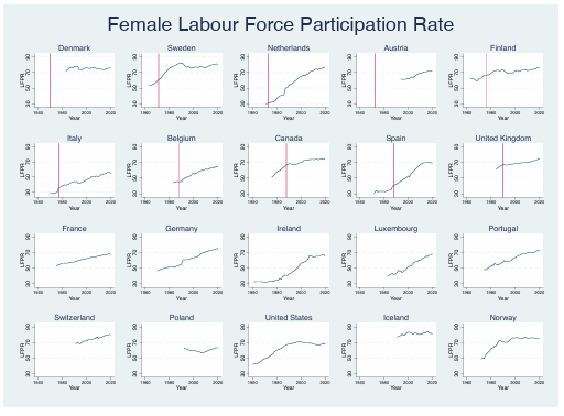
availability in the sample in the earlier decades.
Figure 2: The Female Labour Force Participation Rates in 8 OECD Countries

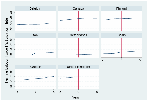
time period that spans 5 years prior to and 5 years following the reform.
Figure 3: The Female Labour Force Participation Rates in 10 OECD Countries

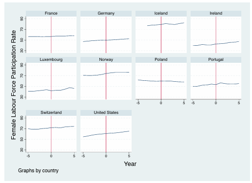
time period. A year is randomly assigned for t = 0, which is detailed in Table 6.
Table 6

assigned period of the reform in Figure 3.
Figure 4: The Labour Force Participation Rates of Women and Men

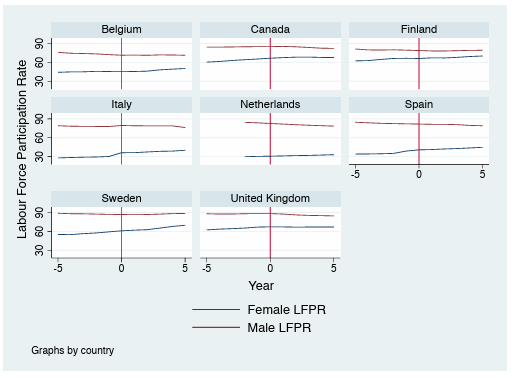
across a 10-year time period that spans 5 years prior to and 5 years following the reform.
Figure 5: The Labour Force Participation Rates of Older and Younger Women

a 10-year time period that spans 5 years prior to and 5 years following the reform.
Figure 6: The Labour Force Participation Rate of Single and Married Women in the UK
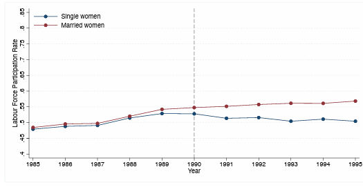

Figure 7: The Labour Force Participation Rate of Single and Married Men in the UK

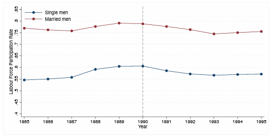
5 years before and after the reform in the UK in 1990.
Table 7: Tax Rates in the UK

marginal rate. In 1994/95, the Married Couple’s Allowance was restricted to a fixed amount (20% of the allowance); it was no longer
available at the taxpayer’s marginal rate. In 1995/96, the Married Couple’s Allowance was available at a flat rate of 15%.
Table 8: Summary Statistics of the Outcome Variables Used in the Event-Study
(a) The Female Labour Force Participation Rates

(b) The Labour Force Participation Rates of Alternative Groups

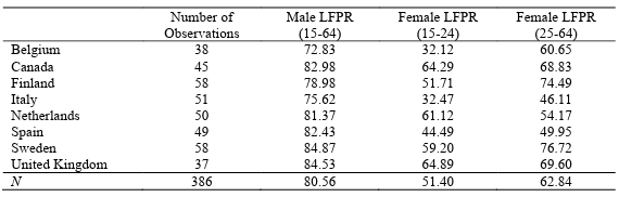
Employment and Labour Market Statistics database.
Table 9: Summary Statistics by Treatment Group and Period
(a) Women in the sample

(b) Men in the sample

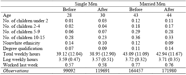
Notes: The table reports the means of the outcome and demographic characteristics including control variables used in the regressions.
The pre-reform period is defined as 1998-1989 and the post-reform period is defined as 1990-1995, since independent taxation was
introduced in 1990. Source: UK LFS data. For total and log weekly hours worked, only those working between 1-75 weekly hours are
included, with standard deviations in parenthesis.
Table 10: Regression Results of The Event-Study of OECD Countries

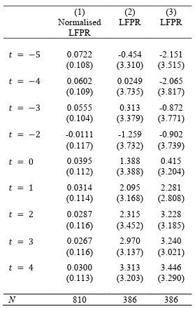
Notes: Robust standard errors in parentheses. * p < 0.05, ** p < 0.01, *** p < 0.001. This table shows the average impact of the various
reforms on the labour force participation rate. The regression coefficients are from the model specified in equation 1. The 3 models
represent the 3 variations of treatment and control group used, which are detailed in Table 5. In column 1, the treatment group is
women aged 15-64 in 8 OECD countries where there is a tax reform of the treatment of married couples and the control group consists
of women aged 15-64 in 10 OECD countries where joint taxation is still in place. The outcome variable of interest is the percentage
change in the labour force participation rate of women relative to the year before the form, so it is normalised at 100 at the year before
the reform !−1. In column 2, the treatment group remains the same and the control group is men aged 15-64 in 8 OECD countries
where there is a tax reform of the treatment of married couples. In column 2, the treatment group remains the same and the control
group is men aged 15-64 in these 8 OECD. In column 3, the treatment group is women aged 25-64 in these 8 OECD countries and the
control group is women aged 15-24 in these countries. In columns 1 and 2, the outcome variable of interest is the difference in labour
force participation rate between the treatment and control group relative to the year before the reform.
Table 12: Regression Results of The Micro-Study of The United Kingdom
(a) Regression Results of the Outcome Variables of Interest for Women

Notes: Robust standard errors in parentheses. * p < 0.05, ** p < 0.01, *** p < 0.001. The base year is the year before the reform (1989).
This table shows the difference in the change between the labour supply of married women and single women. The regression
coefficients reported are from the model specified in equation 2, using 3 different dependent variables for the measures of labour
supply: the participation rate, log weekly hours worked for those in the labour force, and total hours for all women in the sample. This
table also details the baseline regressions and the results after including control variables. Figures 9 and 10 illustrate these outcomes.
(b) Regression Results of the Control Variables for Women
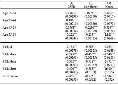
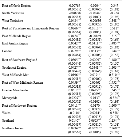


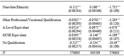
Notes: Robust standard errors in parentheses. * p < 0.05, ** p < 0.01, *** p < 0.001. The base group is white women aged 15-24 with no
children living in the Tyne and Wear region with further education. The measures of labour supply are the participation rate, log
weekly hours worked for those in the labour force, and total hours for all women in the sample.
(c) Regression Results of the Outcome Variables of Interest for Men

Notes: Robust standard errors in parentheses. * p < 0.05, ** p < 0.01, *** p < 0.001. The base year is the year before the reform (1989).
This table shows the difference in the change between the labour supply of married women and single men. The regression coefficients
reported are from the model specified in equation 2, using 3 different dependent variables for the measures of labour supply: the
participation rate, log weekly hours worked for those in the labour force, and total hours for all women in the sample. This table also
details the baseline regressions and the results after including control variables. Figures 9 and 10 illustrate these outcomes.
(d) Regression Results of the Control Variables for Men


Notes: Robust standard errors in parentheses. * p < 0.05, ** p < 0.01, *** p < 0.001. The base group is white men aged 15-24 with no
children living in the Tyne and Wear region with further education. The measures of labour supply are the participation rate, log
weekly hours worked for those in the labour force, and total hours for all women in the sample.
Figure 11: Regression Results by Type of Work

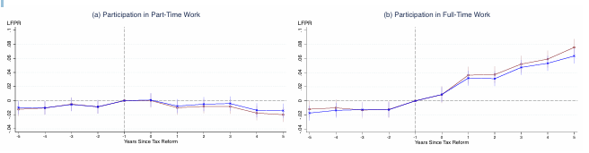
(a) part-time and (b) full-time. The red line gives the results without control variables, and the blue line shows the results after controlling
for observable characteristics.
Figure 12: Regression Results by Education Level

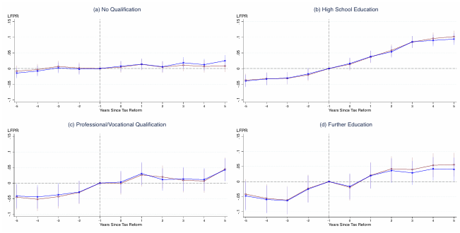
Notes: This shows the regression results for equation 2 by separating the sample by the highest qualification achieved. The dependent
variable is an indicator variable for whether the individual completed paid work in the reference week. The red line gives the baseline
and the blue line shows the effect of controlling for observable characteristics.